Investment Analysis and Portfolio Management

Computation of Expected return for a single Asset.

Return is the required compensation from investing money. It is compensation for deferred consumption. The expected return is the product of probabilities and returns attached to the investment (Kasilingam, n.d.). We are combining the possible outcome from an investment. In the following example, we are calculating the expected return of a single asset a stock. Our probabilities of returns can be based on the state of the economy.

Business Cycles

This pertains to the level of economic activity. We can have a boom period when the economy is at its peak. This is the highest level of economic activity. A recession is a decline in economic activity, Trough or depression is the lowest point in economic activity and expansion or recovery represents the period of economic revival and the general increase in economic activity. There are different signals which explain the level of economic activity.  Investments returns vary with each business cycle.

According to Hull (2018), the expected return is calculated as follows.

Where,

1. E is the probability of return.
2. R is the possible return.

e.g. E(R_i) = [(E­₁) (R₁) + (E₂) (R₂)……(E_n)(R_n)]

The information to calculate the expected return can be computed from historical data.

Returns from investing in a stock.

Probability	Return
0.05	50%
0.25	30%
0.4	10%
0.25	-10%
0.05	-30%

Example Adapted from Hull (2018),

Calculating the expected return or mean. The expected return is the mean. The expected return is the weighted average of the possible returns, where the weight applied to a particular return equals the probability of that return occurring. (Hull, 2018)

 

E(R) =0.05 X (0.50) + 0.25 X (0.30) + 0.40 X( 0.10) + 0.25 X (−0.10) + 0.05 X (−0.30)

= 0.10

= 10%

Risk of Expected Return: Standard deviation of a single asset

According to (Wolski, 2017) risk is the possibility that the actual earning will differ from the expected.  The risk attached to an investment, therefore, needs to be calculated and it is the deviation of the return from the mean. The widely used measure is the standard deviation. Essentially, we want to have a picture of how returns deviate from the average. Our average is our expected return; hence we want to find out how returns are moving around the mean (0.10). The difference between the actual return and the mean (0.10) is the risk

• E=  Probability of return
• E (R)= Expected Return or Mean.

E(R)² = (0.05 × 0.50²) + (0.25 × 0.30²) + (0.40 × 0.10²) + (0.25 × (−0.10)²⁾+(0.05 × (−0.30)²)

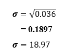
= 0.046

The standard deviation of the annual return is, therefore.

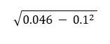
= 0.1897 or

                                                         =18.97%.

Which formula is simple the above and this one?

0.05(0.50-0.10)² +0.25(0.30-0.10)² +0.40(0.10-0.10)²+0.25(-0.10-0.10)² +0.05(-0.30-0.10)²

                                                                                                               

If we are to comment on the results, this investment is risky because a standard deviation of 18.97 is high. Bur high-risk high return investments with high risk have a high return. Risk can be referred to as volatility. How volatile are the returns of an investment or portfolio?

Remember this is the expected return and standard deviation of a single investment.

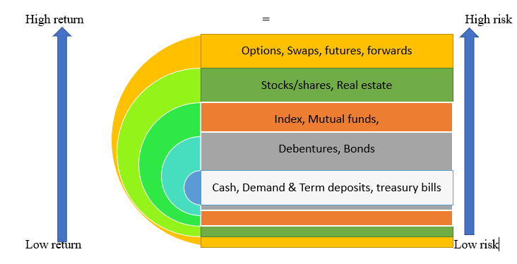
The tradeoff between risk and return.

Now we understand what is expected return and standard deviation. Introducing the concept of a tradeoff between risk and return is essential because for every return there is a risk level associated.  Higher risk investments are high return investments, we are saying investments with higher standard deviation are likely to give a high expected return. Investments with lower risk have lower returns, these investments have a lower standard deviation. Investors are therefore indifferent between high risk and high return, if a higher return is needed more risk must be accepted.  Investors who are indifferent between higher risk and high return and lower risk lower return are known as risk-neutral investors. (Biswas, 1997). However, most investors are risk-averse, they prefer investments with lower returns, with a known level of risk rather than being attracted by higher returns with an unknown level of risk.  As risk increase, risk-averse investors will withdraw their preference over that investment (Montesano, 1990)

            

The expected return of a portfolio of assets.

In Portfolio construction the first issue is to specify the list of securities eligible for selection or inclusion in the portfolio. Secondly, generate the risk-return expectations for these securities. The expected return of a portfolio of assets is simply the weighted average of the return of the individual securities held in the portfolio. The weight applied to each return is the fraction of funds invested in a security that is part of the portfolio. (Reilly and Brown, 2012).

The formula for Expected return.

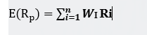
Once we have information regarding individual assets returns or individuals investments we are now thinking in terms of the combined set of investments or a portfolio.

• E(Rp)= Expected return of the portfolio
• W_i = Proportion of funds invested in security i
• Ri = Expected return of security i
• n = Number of securities in the portfolio

Example

 

 

 

 

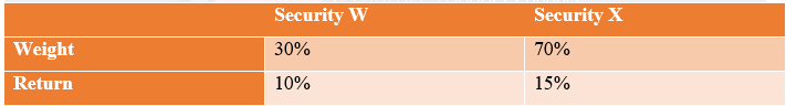
Weights

Security W: (W_w)                      30%

Security X: (W_x)                        70%

Returns

Security W: (R_w)                      10%

Security X: (R_x)                        15%

A two-security portfolio:  =W_w (R_w) + W_x (R_x)

= (0.3) (10) + (0.7) (15) = 13.5%

 Bibliography

1. Hull, J., 2018. Risk management and financial institutions, Fifth edition. ed. Wiley, Hoboken, NewJersey.
2. Reilly, F.K., Brown, K.C., 2012. Investment analysis & portfolio management, 10th ed. ed. South-Western Cengage Learning, Mason, OH.
3. Kasilingam, D.R., n.d. Reader, Department of Management Studies, Pondicherry University Puducherry 292.
4. Montesano, A., 1990. On the definition of risk aversion. Theor Decis 29, 53–68. https://doi.org/10.1007/BF00134104
5. Biswas, T., 1997. Risk Aversion, in: Biswas, T. (Ed.), Decision-Making under Uncertainty. Macmillan Education UK, London, pp. 19–29. https://doi.org/10.1007/978-1-349-25817-8_2
6. Business Cycle Phases: Defining Recession, Depression, Expansion [WWW Document], n.d. URL https://www.business-case-analysis.com/business-cycle.html (accessed 3.1.21).
7. Wolski, R., 2017. Investment risk in real estate and other financial assets, in: 24th Annual European Real Estate Society Conference. Presented at the 24th Annual European Real Estate Society Conference, European Real Estate Society, Delft, Netherlands. https://doi.org/10.15396/eres2017_83